3. Plot results#
This section introduces all the plotting functions that help visualise the queried observations:
3.1 - Plot an overview of the observations (alminer.plot_overview)
3.2 - Plot an overview of a given line in the observations (alminer.plot_line_overview)
3.3 - Plot observed frequencies in each band (alminer.plot_bands)
3.4 - Plot observations in each band (alminer.plot_observations)
General notes about the plotting functions:
Most of the plotting functions have the option to mark frequencies of CO, 13CO, and C18O lines by toggling mark_CO=True. A redshift can be provided by setting the z parameter that will shift the marked frequencies accordingly.
Most of the plotting functions have the option to mark a list of frequencies. A redshift can be provided by setting the z parameter that will shift the marked frequencies accordingly.
Plots can be saved in PDF format by setting the savefig parameter to the desired filename. Figures are saved in a subdirectory called ‘reports’ within the current working directory. If the directory doesn’t exist, it will be created.
To avoid displaying the plot (for example to create and save plots in a loop), set showfig=False.
Load libraries & create a query
To explore these options, we will first query the archive using one of the methods presented in the previous section and use the results in the remainder of this tutorial.
[1]:
import alminer

observations = alminer.keysearch({'science_keyword':['Galaxy chemistry']},
                                 print_targets=False)
================================
alminer.keysearch results
================================
--------------------------------
Number of projects = 54
Number of observations = 376
Number of unique subbands = 1288
Total number of subbands = 1501
Total number of targets with ALMA data = 79
--------------------------------
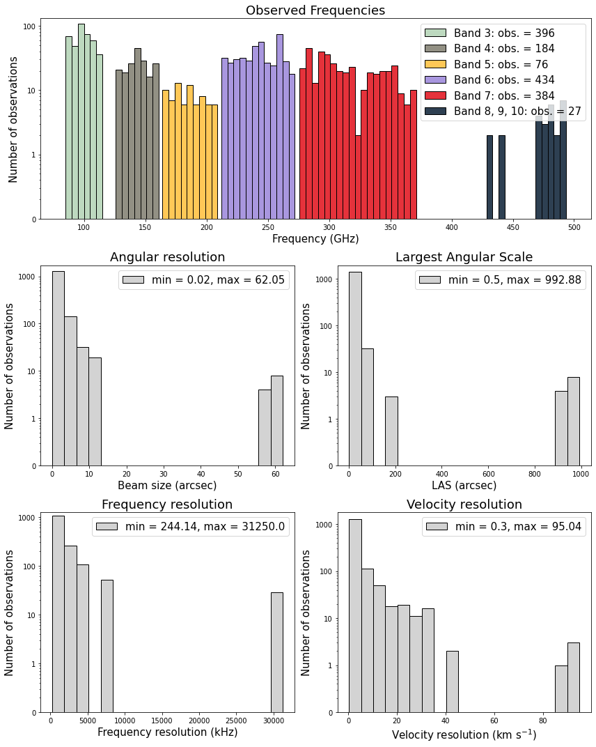
3.1 Plot an overview of the observations#
The alminer.plot_overview function plots a summary of the observed frequencies, angular resolution, largest angular scales (LAS), and frequency and velocity resolutions.
Note: The histogram of observed frequencies displays the distribution of central frequencies and also depends on the choice of binning. To get an overview plot for a specific frequency, use alminer.plot_observations and alminer.plot_line_overview (see examples below).
Example 3.1.1: plot an overview of the observations and save the figure#
[2]:
alminer.plot_overview(observations, savefig='alma_galaxy_chemistry')
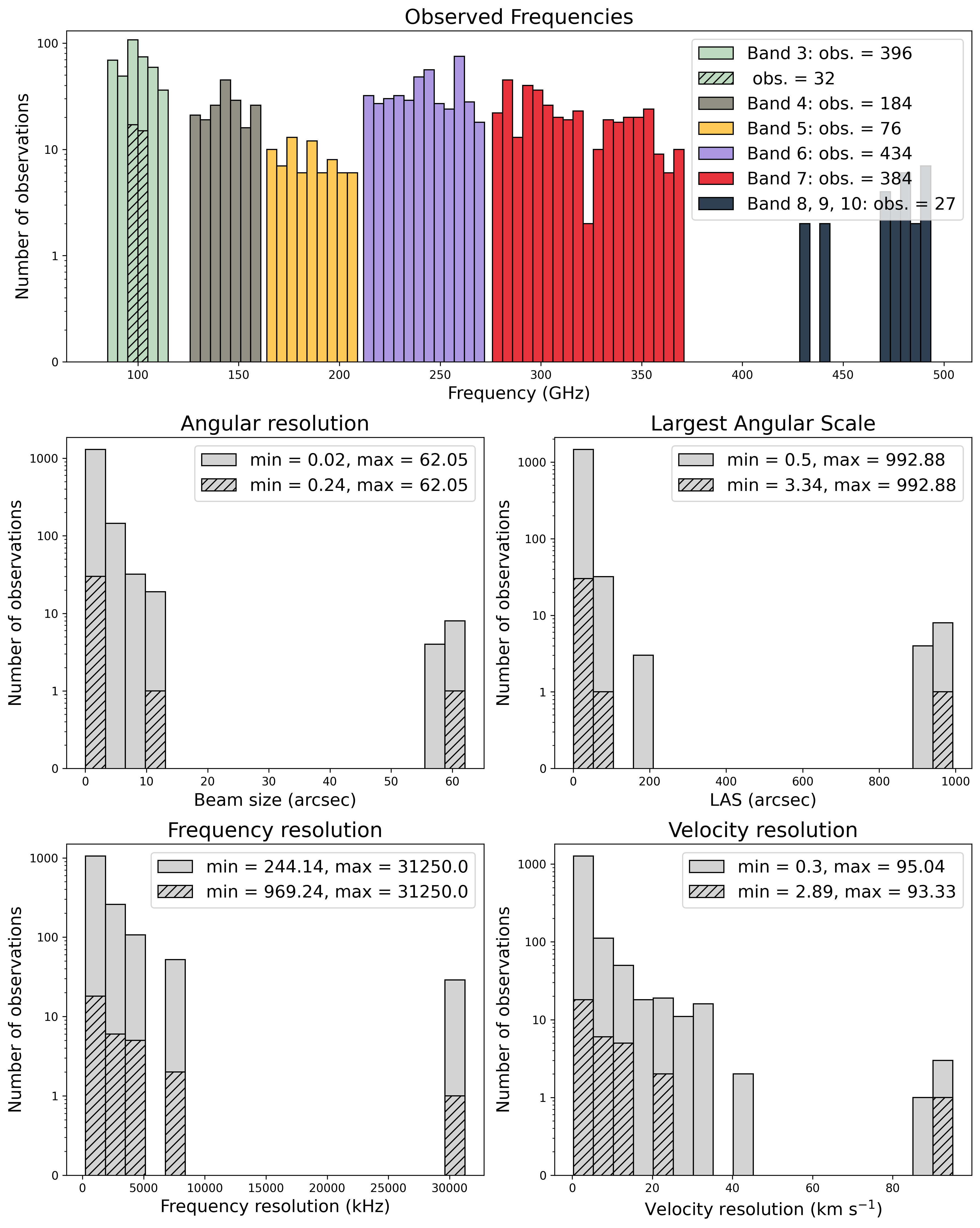
3.2 Plot an overview of a given line in the observations#
The alminer.plot_line_overview function creates overview plots of observed frequencies, angular resolution, LAS, frequency and velocity resolutions for the input DataFrame, and highlights the observations of a give frequency (redshift if the z parameter is set) specified by the user.
Example 3.2.1: plot an overview of the observations and highlight observations at a particular frequency#
[3]:
alminer.plot_line_overview(observations, line_freq=100.0)
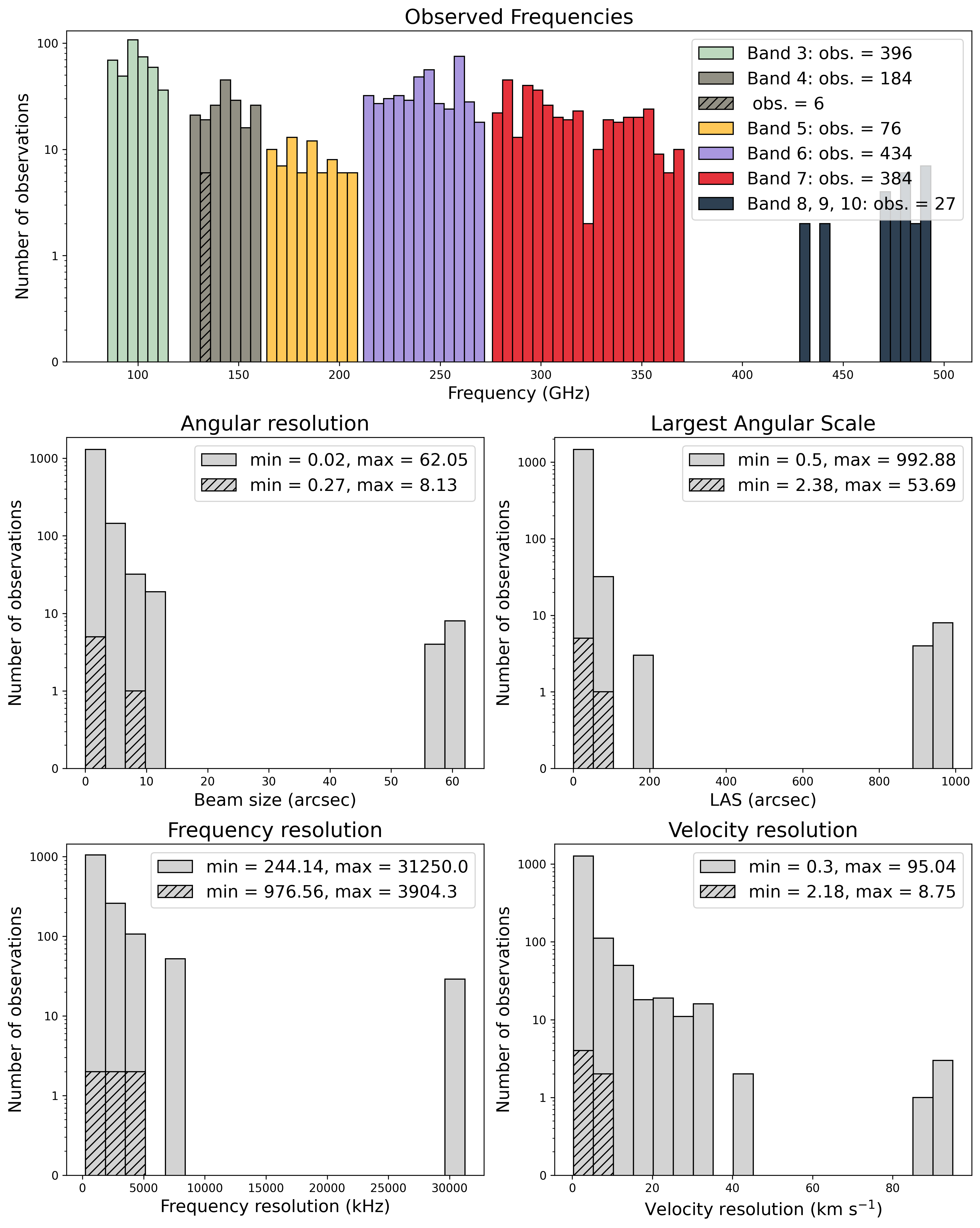
Example 3.2.2: plot an overview of the observations and highlight observations at a redshifted frequency#
[4]:
alminer.plot_line_overview(observations, line_freq=400.0, z=2)
3.3 Plot observed frequencies in each band#
The alminer.plot_bands function creates detailed plots of observed frequencies in each band.
Example 3.3.1: plot observed frequencies in each band and mark redshifted CO lines#
[5]:
alminer.plot_bands(observations, mark_CO=True, z=0.5)
Example 3.3.2: plot observed frequencies in each band and mark frequencies of choice#
[6]:
alminer.plot_bands(observations, mark_freq=[106.5, 245.0, 366.3])
3.4 Plot observed frequencies in each band#
The alminer.plot_observations function creates a detailed plot of observations in each band showing the exact observed frequency ranges. Observation numbers are the input DataFrame’s index values.
Example 3.4.1: plot observed frequencies in each band and mark CO lines#
[7]:
alminer.plot_observations(observations, mark_CO=True)
Example 3.4.2: plot observed frequencies and mark frequencies of choice#
[8]:
alminer.plot_observations(observations, mark_freq=[106.5, 245.0, 366.3])
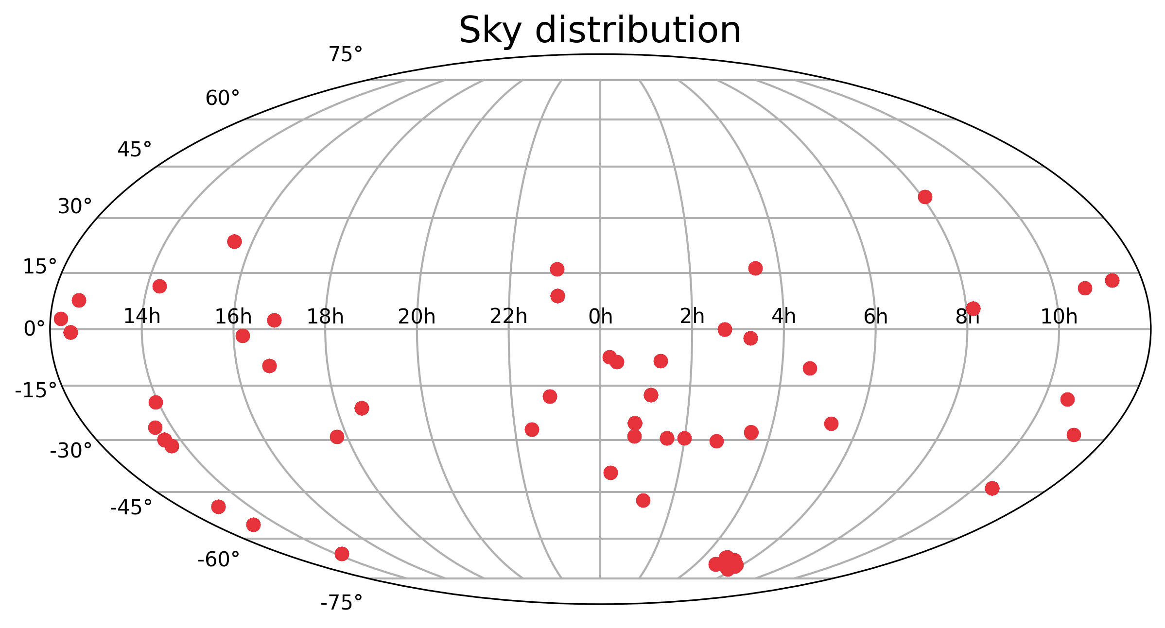
3.5 Plot sky distribution#
The alminer.plot_sky function creates a plot of the distribution of targets on the sky.
Example 3.5.1: plot sky distribution#
[9]:
alminer.plot_sky(observations)